About goflow: 
This repository is all about simulating flow driven pruning in biological flow networks.
##  Introduction
Biological transport networks are dynamic systems developing constantly, to be found where ever you may look. The common, if not universal feature is that all such networks grow from a redundant initial plexus (a rudimentary network) into their final structure on the onset of flow. E.g. see the slime mold physarum in the little movie below, rebuilding the Tokyo railway system from scratch (Tero et al, Rules for Biologically Inspired Adaptive Network Design, Nature, 2010).
<br>

![physarum](https://raw.githubusercontent.com/felixk1990/go-with-the-flow/gh-pages/gallery/tokyoPhysarum.gif)

<br>

![katifori](https://raw.githubusercontent.com/felixk1990/go-with-the-flow/gh-pages/gallery/ronellenfitsch.png)

<br>
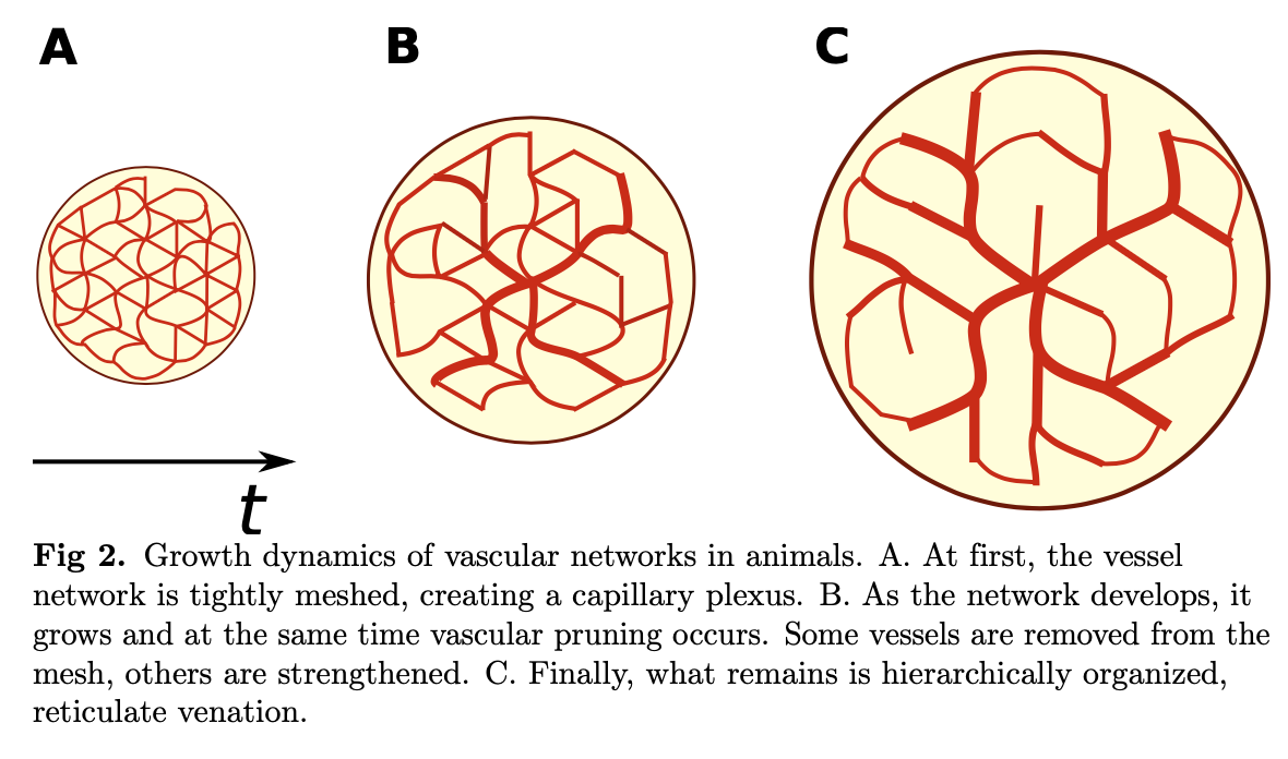
[From: Ronellenfitsch et al, arXiv:1707.03074v1]<br>

This module 'goflow' is the final of a series of python packages encompassing a set of class and method implementations for a kirchhoff network datatype, in order to to calculate flow/flux on lumped parameter model circuits and their corresponding adaptation. The flow/flux objects are embedded in the kirchhoff networks, and can be altered independently from the underlying graph structure. This is meant for fast(er) and efficient computation and depends on the packages 'kirchhoff','hailhydro'.

What does it do: Modelling morphogenesis of capillary networks which can be modelled as Kirchhoff networks, and calculate its response given flow q/ pressure dp/flux j based stimuli functions. We generally assume Hagen-Poiseulle flow and first order solution transport phenomena Given the radii r of such vessel networks we simulate its adaptation as an ODE system with <br>

<img src="https://render.githubusercontent.com/render/math?math=\dot{r}_i (t) = f_i( \lbrace r \rbrace, \lbrace q \rbrace, \lbrace j \rbrace, ... ) ">

The dynamic system f is usually constructed for a Lyapunov function L with <br>

<img src="https://render.githubusercontent.com/render/math?math=L = \sum_i \alpha_1 p_i^2r_i^4 %2B \alpha_0 r_i^2 %2B+...">

such that we get <br>
<img src="https://render.githubusercontent.com/render/math?math=f_i( \lbrace r \rbrace, \lbrace q \rbrace, \lbrace j \rbrace, ... )= -\frac{dL}{dr_i} ">

The package not only includes premade Lyapunov functions and flow/flux models but further offers custom functions to be provided by the user.
##  Installation
pip install kirchhoff hailhydro goflow
##  Usage
First you have to create your rudimentary circuit/ flow network which you want to evolve later:
```
import numpy as np
import kirchhoff.circuit_init as kfi
from goflow.adapter import init_ivp as gi

init_flow=dict(
    crystal_type='triagonal_planar',
    periods= 3,
)
C = kfi.initialize_circuit_from_crystal(**init_flow)

pars_src = {
    'modesSRC': 'root_geometric'
}
pars_plx = {
    'modePLX':'default',
}
pars_model = {
    'alpha_0':1.,
    'alpha_1':1.
}

morpheus = gi.morph_dynamic(C, 'murray', [pars_model, pars_src, pars_plx])
morpheus.evals = 200

cnd = morpheus.flow.circuit.edges['conductivity']
cnd_scale = morpheus.flow.circuit.scales['conductance']

sp = {
    't0': 1e-05,
    't1': 4.,
    'x0': np.power(cnd/cnd_scale,0.25)*0.1,
}
nsol = morpheus.nlogSolve((sp['t0'],sp['t1']), sp['x0'])

dataPoints = zip(nsol.t,nsol.y.transpose())
murrayModel = morpheus.model
args = murrayModel.solver_options['args']
cost = [murrayModel.calc_cost_stimuli(t, y, *args)[0] for t, y in dataPoints]
```

When you are done, plot the plexus, dynamics of vessel development and final structure as:
```
aux = {
    'color_nodes': ['#030512'],
    'colormap': ['RdPu'],
}
morpheus.flow.circuit.edges['conductivity'] = np.round(nsol.y.transpose()[0],5)
lw = morpheus.flow.circuit.edges['conductivity']
morpheus.flow.circuit.edges['flow_rate'], dP = morpheus.flow.calc_configuration_flow()
morpheus.flow.circuit.edges['flow_rate'] = np.round(np.absolute(morpheus.flow.circuit.edges['flow_rate']),5)
fig = morpheus.flow.circuit.plot_circuit(linewidth = [10.*lw], color_edges = [lw], **aux)
fig.show()

morpheus.flow.circuit.edges['conductivity'] = np.round(nsol.y.transpose()[-1],5)
lw = morpheus.flow.circuit.edges['conductivity']
morpheus.flow.circuit.edges['flow_rate'], dP = morpheus.flow.calc_configuration_flow()
morpheus.flow.circuit.edges['flow_rate'] = np.round(np.absolute(morpheus.flow.circuit.edges['flow_rate']),5)
fw = morpheus.flow.circuit.edges['flow_rate']

fig = morpheus.flow.circuit.plot_circuit(linewidth = [5.*lw], color_edges = [lw], **aux)
fig.show()

fig = go.Figure()
for i, ys in enumerate(nsol.y):

    e = morpheus.flow.circuit.edges['label'][i]
    fig.add_trace(
        go.Scatter(
            x= nsol.t,
            y= ys,
            mode='lines',
            line=dict(color='rgba(0,0,255,0.1)'),
            name=f'vessel {e}'
        )
    )

fig.update_xaxes(type="log")
fig.show()
```
<iframe src="https://felixk1990.github.io/go-with-the-flow/plexus.html" title="plexus" width="100%" height="600" style="border:none;"></iframe><br>
<iframe src="https://felixk1990.github.io/go-with-the-flow/dynamics.html" title="dynamics" width="100%" height="800" style="border:none;"></iframe><br>
<iframe src="https://felixk1990.github.io/go-with-the-flow/final.html" title="final" width="100%" height="600" style="border:none;"></iframe><br>

If you like you may generate animations just as easily, e.g. see the examples in the gallery section:

![updated1](https://raw.githubusercontent.com/felixk1990/go-with-the-flow/gh-pages/gallery/murray_triagonal_plexus.gif)<br>
![updated2](https://raw.githubusercontent.com/felixk1990/go-with-the-flow/gh-pages/gallery/murray_triagonal_dynm.gif)<br>

Further examples and recipes: [![Binder](https://mybinder.org/badge_logo.svg)](https://mybinder.org/v2/gh/felixk1990/go-with-the-flow/examples)
##  Requirements
``` pandas ```,``` networkx ```, ``` numpy ```, ``` scipy ```, ``` kirchhoff ```, ``` hailhydro ```, ```plotly```

## Acknowledgement
* Pre-customized models presentend and implemented here as given by:
    *  Murray, The Physiological Principle of Minimum Work, 1926
    *  Katifori et al, Damage and Fluctuations Induce Loops in Optimal Transport Networks, 2010
    *  Corson, Fluctuations and Redundancy in Optimal Transport Networks, 2010
    *  Hu and Cai, Adaptation and Optimization of Biological Transport Networks, 2013
    *  Kramer and Modes, How to pare a pair: Topology control and pruning in intertwined complex networks, 2020

```goflow``` written by Felix Kramer